Ryerson Computer Science MTH820: Image Analysis
(go back)Sampling & Quantization
Sampling is the division of the domain, while quantization is the division of the range
Matlab
Some general matlab functions and code
					% show the image with pixel info
					imshow('moon.tif'), impixelinfo
					% reads the image into image1 variable
					image1=imread('moon.tif');
					% shows all the variables
					whos
					% displays 2 images in a figure
					figure, subplot(1,2,1), imshow(image1),
						subplot(1,2,2), imshow(image2)
					% for following subplot...
					% m = # of rows
					% n = # of columns
					% p = position where the image will go
					subplot(m,n,p)
						% creates an image, imgDbl that uses
						% 8 bytes per pixel
						f = double(imageUint8)
						% converts to a matrix of doubles between
						% 0 and 1
						f2 = im2double(f)
						imwrite(f2, 'myPicture.jpg', 'quality', 50)
						[rows, cols] = size(f2)

						%loop through specific values:
						someVals = [1 3 4 6 10]
						for k = 1:length(someVals)
							theVal = someVals(k)
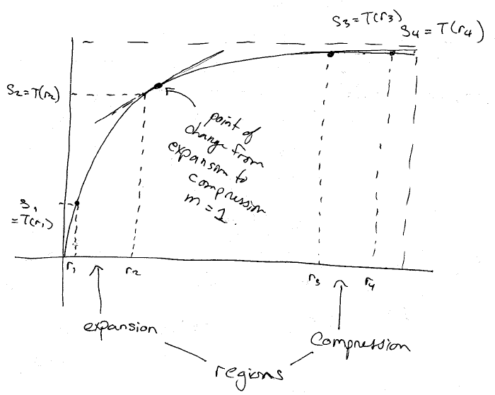
Intensity Transformations
An image transformation function, in general, is some function that is used to adjust the intensity values of the pixels in an image. Depending on the function, all or only some of the pixels will be adjusted. These functions are used for applications such as contrast improvement.
Histogram Equalization
The purpose is to correct a poor image pixel intensity histogram. The ideal histogram shape is a flat line that evenly covers all intensity values. This would imply that every intensity is used equally among all the pixels. As opposed to a histogram that is narrow (bunched in one region) - this indicates that all the pixels use only a small subset of the possible intensity values. This means the contrast is poor.
Histogram Matching
Matlab can attempt to adjust the image pixel intensity histogram and match it with a histogram provided by the user.
Matlab
					g = histeq(f, hgram)
					hgram = (hgram(1), hgram(2), ..., hgram(256))
					% Useful histogram shape: gauss curve:
					% 	$g(x) = A \cdot e^{\frac{-(x-m)^2}{\sigma^2}}$
					% example of generating a gauss-based histogram
					x = linspace(0,1,256); 	% evenly spaced array
					m = 1/2; s = 0.1; 		% params for gauss
					y = exp(-((x-m)/s).^2); %gauss fmla
					% scale down so the sum of everything is 1
					y = y / sum(y);
Histogram curve in above code: $g(x) = A \cdot e^{\frac{-(x-m)^2}{\sigma^2}}$
Spatial Filtering
Blurring
Takes the average of a set of "neighbouring" values and applies that to the focal pixel. For better results can use a weighted average provided by the Gaussian function
$\Sigma\ w_{ij} = 1$ (must always be true)
Matlab
						g = imfilter(f, w)
						w = fspecial('average', N)
						w = fspecial('average', [M N])
						w = fspecial('gaussian', size, sigma)
Sharpening: Unsharp Masking
The idea here is to basically subtract the blur (the mask) from the image in order to sharpen it.
Matlab
						mask = f - blur(f);
						% (k provides some adjustment or control over the blur)
						g = f + mask*k;
Sharpening: Laplacian
Sample Laplacian filters:
$\Sigma\ w_{ij} = 0$ (must always be true)
$\begin{pmatrix} 0 & 1 & 0 \\ 1 & -4 & 1 \\ 0 & 1 & 0 \end{pmatrix} \begin{pmatrix} 1 & 1 & 1 \\ 1 & -8 & 1 \\ 1 & 1 & 1 \end{pmatrix}$
Matlab
						w = fspecial('laplacian', 0);
						f = im2double(imread(image));
						g = imfilter(f, w); % this gives the "details"
						h = f - g
						% the brackets scale the image to
						% the viewable range of values
						imshow(h, []);
Sharpening: Laplacian of the Gaussian (LoG)
This technique involves blurring the image first, then sharpening. Starting with a mild blurring is one way to remove noise from the original image so that the sharpening doesn't amplify that noise in addition to sharpening the features
LoG math function
$\frac{-1}{2 \sigma^2}\left(1 - \frac{2^{(x^2 + y^2)}}{\sigma^2} \right)e^{-\frac{(x^2 + y^2)}{2\sigma^2}}$
Matlab
						f = im2double(imread('image'))
						w = fspecial('log', N, sigma)
						g = imfilter(f, w)
						h = f - g
Geometric Transformations
Transformations result in pixels being relocated, and often the boundaries of the image matrix changing
Affine/Projective
An affine transformation results in an image that is scaled, mirrored, translated, or skewed (maybe more). Projective transformations provide a change in apparent depth of some portion of the image. They both use a matrix in the form: $\begin{pmatrix} a & b & e \\ c & d & f \\ b_1 & b_2 & 1 \end{pmatrix}$
Where a = x scaling, b = y shearing, c = x shearing, d = y scaling, b1 & b2 offer translation, and e & f are used for projection, but set to 0 for non-projection affine
Rotation
Rotation (clockwise) uses an affine transformation matrix in the following form: $\begin{pmatrix} cos\Theta & sin\Theta & 0 \\ -sin\Theta & cos\Theta & 0 \\ 0 & 0 & 1\end{pmatrix}$
Aside: Interpolation
In transforming images, resultant calculated pixel locations are not always exact integers, but they need to be coerced into integer locations using some form of interpolation. There are three main ones, from simplest to most complex: Nearest neighbour, Bilinear, Cubic Polynomial. The default in Matblab is Bilinear, but nearest neighbour may work better in many cases.
Matlab
					% here T is a standard matrix in a form mentioned above
					tform = maketform('affine', T [, 'FillValue', alpha])
					% FillValue with alpha is optional, but fills any empty
					% space created at the edge of the matrix with some intensity value give by $\alpha$
					g = imtransform(f, tform)
Point-based Registration
Image Registration is the transformation of a given image to conform in some way to a base image. Control points are selected on the base image, then the input image is transformed in a way that the same points are found on as those selected on the base image, and they points are moved to be in the same position as the base image. Used in applications where the subject of the image needs to be in a consistent location in the frame.
Matlab
					% this brings up a nice interface for selecting points then use file->export points to workspace
					cpselect(input_img, base_img)
					% for TransformationTypes  Affince and Projective...
					% P = input control points, Q = base image control points
					tform = cp2tform(P, Q, 'TransformationType')
					% imtransform can return x and y coords info which is useful
					% for plotting.Then use impixelinfo to find where to crop
					[ f1, xdata, ydata ] = imtransform(f, tform)
					% how to plot orig and translated together
					imshow(f, 'XData', xdata, 'YData', ydata);hold on;
					imshow(f1);axis on;axis auto;
Area-based Registration
Here we choose a template, which is a section of an image, that is used to compare against another image to see if there is a matching section. The matching process is called normalized cross-correlation.
					% we can choose a template from an existing image, like g. This just graphs a square of image g.
					template = g(10:20, 10:20)
					% the template is then used for cross-correlation against one of the images.  The max value(s)
					% indicate the highest correlation (probably a match)
					g = normxcorr2(template, f)
					dx = ... % find diff between x in one img and t'other
					dy = ... % find diff between y in one img and t'other
					tform = maketform('Affine', [1 0  0; 0 1 0; dx dy 1]);
					% yadda
Morphological Image Processing
Determine various properties of a image. Often used in identifying or counting objects in an image. The image must be turned in a "boolean" image (basically B&W) so regions can be recognized. Thresholding is used to convert to boolean.
Thresholding
Here we must choose a threshold, $t$, for converting
$g(x,y) = \begin{cases} 0 & if\ f(x,y) \leq t \\ 1 & if\ f(x,y) \gt t \end{cases}$
Then g = f > t.
Erosion (thining) $A \ominus n B$
For a given structuring element (often a square matrix), the image area is reduced in size given the logical rule that the entire structuring element must be a subset of the area in question. We can repeat this process n-many times (where n is ≥ 1, but usually is just 1).
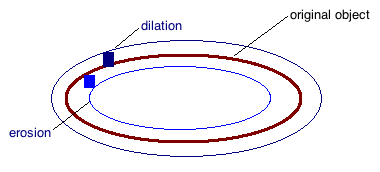
Dilation (thickening) $A \oplus n B$
For a given structuring element, the image area is increased in size given the logical rule that the area can be made to occupy any area such that the any part of the structuring element intersects the original area. Img below shown with two square structuring elements. We can repeat this process n-many times (where n is ≥ 1, but usually is just 1).
Matlab
					% where 'a' is a binary img, and 'b' is a structuring element
					c = imerode(a, b)
					% or...
					c = imdilate(a, b)
					% and to create an SE:
					b = strel('Square', 3) % creates a 3x3 square structuring el
Opening: $A \circ B = (A \ominus n B) \oplus n B$
If we apply erosion followed by dilation, it is called opening of A by B. Properties of this include:
- smooths contours from the inside
- breaks small bridges
- eliminates protrustion
- $A \circ B \subset A$
c = imopen(A,B)
Closing $A \bullet B = (A \oplus n B) \ominus n B$
If we apply dilation followed by erosion, it is called closing of A by B. Properties include:
- smooths contours from the outside
- fills breaks & holes
- joins nearby segments
- $A \subset A \bullet B$
c = imclose(A,B)
Hole Filling
$X_0$ = zero image with a 1 in each hole
$X_1 = (X_0 \oplus B) \cap A^C$
$X_2 = (X_1 \oplus B) \cap A^C$
... stop when $X_{k+1}$ = $X_k$. Now we have a set of inverted holes. Can add these to the original image to fill in its holes
Or, just use imfill:
gFilled = imfill(g_swissCheese, 'holes')
Component Finding
same procedure as hole finding/filling, except to find the components we intersect against $A$ instead of $A^C$.
Sample Component Finding & Counting Code
				function xnew = findComponent( i, j, f )
				    xnew = zeros(size(f));
				    xold = xnew;
				    xnew(i,j) = 1;
				    b = [ 0 1 0; 1 1 1; 0 1 0 ];
				    while any(xold(:) ~= xnew(:))
				        xold = xnew;
				        xnew = imdilate(xnew, b) & f;
				    end
				end
Morphological Reconstruction
This allows us to reconstruct components of an image that were possibly removed during intensive erosion. Same algorithm as component finding except initial point $X_0$ is a set, or matrix, of points.
Typical way to find F: erosion of the original image $A \ominus n B$
Matlab:
imreconstruct(F, A, Connectedness) % Connectedness is 4 or 8
Greyscale Morphology
The following tools are useful in greyscale morphology before thresholding
Greyscale Opening
Darkens the image in a controlled way
Tophat Transform
This is the opening of the image f, subtracted from f: $f - (f \circ B)$
Greyscale Closing
Lightens the image in a controlled way
Bottomhat Transform
This is the image, f, subtracted from the closing of f: $(f \bullet B) - f$
Image Segmentation
Dividing up an image into distinct regions based on some criteria, like qualities of edges or regions. Additional techniques often need to be employed such as pre-segmentation sharpening (and pre-segmentation-sharpening blurring).
Edge-based segmentation
In the following matlab sample, the extra 't' output parameter is matlab's attempt at finding a reasonable threshold if you do not provide the optional T input parameter. You can use this output param as a guide for choosing your own appropriate input T parameter
		[ g, t ] = edge(f, method, T)
		[ g, t ] = edge(f, 'log', T, sigma)
		[ g, t ] = edge(f, 'canny', [Tlow, Thi], sigma)
Region Based Segmentation
Region-based segmentation (by inspection)
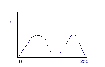
With region-based segmentation, we segement the image based on a threshold obtained by the intensity of particular regions. The approach essentially boils down to using a histogram. Depending on the image, the threshold can be ascertained simply by inspecting it (in the case of two distinct humps), or by using a more complex algorithm like Otsus. For an image with a histogram like the one below, we can simply choose the threshold by inspecting the historgram and choosing the low point between the humps.
Region-based segement with Otsus
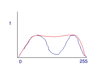
For image histograms that lack the distinction between two regions, we need to use a more powerful technique. The Otsus method uses a statistical algorithm to find the optimal threshold. This will work for both simple and relatively complicated histograms. The red line in the image below is the actual histogram, while the blue humps are the "hidden" truly distinct regions. Otsus can uncover the distinct humps (in most cases).
		%Otsus is graythresh (returns value from 0 to 1)
		T = graythresh(f)
		g = f > T*256.
Three-Region Segmentation
For segmenting into three regions, if possible, just look at the histogram. If the histogram does not have the necessary three distinct humps, then blurring is one option.