Ryerson Computer Science CPS616: Analysis of Algorithms
(go back)Smalltalk
Pseudo variables
- nil, true, false, self, super
Loops
				10 timesRepeat: [ ... ].
				[ x < 10 ] whileTrue: [ ... ].
				1 to: 10 do: [ :i | ... ].
Iterating
				myArray do: [:item| ... ].
				myArray doWithIndex: [:item :idx | ... ].
Equality
				> "greater than"
			    <=  "less than"
			    =  "equal to in value"
			    ~= "not equal in value"
			    >= "greater than or equal to"
			    <= "less than or equal to"
			    == "is the same object"
Order Notation
Given $f(n)$ and $g(n)$:
- Big-O: $f = O(g)$ means f grows no faster than g
- Big-$\Omega$: $f = \Omega(g) ~~ \Rightarrow ~~ g = O(f)$ (opposite of Big-O)
- Big-$\Theta$: $f = \Theta(g) ~~ \Rightarrow ~~ f = O(g)$ AND $f = \Omega(g)$ (both!)
Order Notation Rules
- Multiplicative constants can be ignored [$55n^2 ~~ same~as ~~ n^2 ~~ same~as ~~ 0.01n^2$]
- Higher powers dominate [$n^4 ~ > ~ n^2 ~ > ~ n ~ > ~ n^{1/2}$]
- Any exponential dominates polynomials [$1.5^n > n^4 ~~except~~ 0.5^n$]
- larger exponential bases dominate [$3^n > 2^{5n}$]
- any polynomials dominate logarithms [$n^2 > n\cdot log(n) > n > log(n^2) > log^2(n)$]
How to compare two algorithms (Jeff's Procedure)
To determine the complexity relationship between $f(n)$ and $g(n)$, take the limit (as n approaches $\infty$) of the division of the two algorithms: $\lim_{x \to \infty}(f(n)/g(n))$. If the limit arrives at a constant, then $f = O(g)$. If the result goes to $\infty$, then $f = \Omega(g)$. If the result is a constant, AND the result of the limit of $g(n)/f(n)$ is also constant, then $f = \Theta(g)$.
Careful when evaluating these limit problems! Use the order notation rules to determine what dominates the limit so that terms can be ignored
Ex How large a problem can be computed with these two algorithms?
Solution:
1) convert 16GB to bits (in-class example was different and probably incorrect).
$16GB = 16 \cdot 1024MB$
$~~~~~~~~~ = 16 \cdot 1024 \cdot 1024KB$
$~~~~~~~~~ = 16 \cdot 1024 \cdot 1024 \cdot 1024B$
$~~~~~~~~~ = 16 \cdot 1024 \cdot 1024 \cdot 1024 \cdot 8 ~bits$
$~~~~~~~~~ = 8 \cdot 16 \cdot 1024 \cdot 1024 \cdot 1024 ~bits$
$~~~~~~~~~ = 2^3 \cdot 2^4 \cdot 2^{10} \cdot 2^{10} \cdot 2^{10} ~bits$
$~~~~~~~~~ = 2^{37} ~bits$
2) Solve for $n$ for each algorithm:
Alg1:
$4n^2 = 2^{37}$
$~~n^2 = \dfrac{2^{37}}{4}$
$~~n = 2^{17.5}$
Alg2:
$1024n = 2^{37}$
$n = \dfrac{2^{37}}{2^{10}}$
$n = 2^{27}$
(this one can do more!)
Complexity of Common Problems
Arithmetic problems on binary numbers, s.t. n represents the number of bits
Problem | Complexity | Explanation |
|---|---|---|
Addition | $O(n)$ | single summation operation one each bit (assumes two numbers of same bit length) |
Multiplication | $O(n^2)$ | uses recursion n times, each time performs K operations on each bit (kn), resulting in $n \cdot kn \Rightarrow n^2$ |
Algorithms with Numbers
Modular Arithmetic
Recall congruence relation: $a \equiv b (mod\ n)$
if a - b is a multiple of n
Calculating GCD using Euclid's Method
gcd(a, b) = { if b == 0 return a else gcd(b, a mod b ) }
Calculating GCD using Prime Factorization
divide up both the numbers until you can represent them only with primes (like 2x2x3x5, etc), then find any overlapping numbers between the two sets, then take the product of all the overlapping numbers)
Eg, gcd(18, 84):
- 18 = 3x3x2
- 84 = 7x3x2
- So the gcd is 2x3 = 6
Inverse Mod
Using modular arithmetic, find the following inverse: 20 (mod 79). Essentially we need to find integer values that satisfy: 20(x) + 79(y) = 1. Sometimes it can be seen by inspection, as with this example, obviously 20(4) + 79(-1) = 1. But when the factors are less obvious, we may need to check that there is indeed an inverse at all by verifying if gcd(79,20) is equal to 1. If it is equal to 1, then there is some inverse, if not, then there is no inverse.
Algorithm for Primality Testing
Choose positive integers: $a_1, a_2, ... a_k \lt N$ at random
if $a_i^{N-1} \equiv$ 1 (mod N) for all i = 1, 2, .., k: return TRUE, else FALSE
Pr(alg1 returns TRUE when N is not prime) ≤ $\dfrac{1}{2^k}$
RSA Crypto Systems: Public Key Encryption
Alice & Bob overview:
- Bob chooses his public & secret keys:
- he stats by picking two large random primes, p and q
- his public key is (N, e) where N = pq and e is relatively prime to (p-1)(q-1)
- his secret key is d, the inverse of e modulo (p - 1)(q - 1), computed using the extended Euclid algorithm
- Alice wishes to send msg x to Bob
- she looks up his public key (N, e) and sends him y = ($x^e$ mod N), computed using a modular exponentiation algorithm
- Bob decodes the msg by computing $y^d mod N$
RSA hinges on this assumption: given N, e, and y = $x^e$ mod N, it is computationally intractable to determine x
Divide & Conquer Algorithms
- Break a problem up into subproblems that are themselves smaller instances of the same type of problem
- Recursively solve the subproblems
- Appropriately combine their solutions
Multiplication
Technique splits binary numbers into two to apply a special multiplication that requires less recursive operations (only 3)
$T(n) = 3T(n/2) + O(n)$ --> which is $O(n^{1.59})$
Recurrence Relations - Master Theorem
Master Theorem: $T(n) = a\cdot T(\lceil n/b \rceil) + O(n^d)$
... for constants a > 0, b > 1 and d ≥ 0, then:
$T(n) = \begin{cases} O(n^d), & if\ d \gt log_ba \\ O(n^d\ log\ {n}), & if\ d = log_ba \\ O(n^{log_b\ {a}}), & if\ d \lt log_ba \\ \end{cases}$
Where:
- $a$ is the number of branches we are dividing the algorithm into (to actually work on)
- $b$ is the size of the sub-problem
- d is the the amount of time spent partitioning and re-combining the result
Merge Sort: $O(nLog n)$
Median Selection: $O(n)$
Graph Decomposition
Exploring all nodes of a graph from a designated starting point.
Depth-First Search
Depth-first search (DFS) is an algorithm for traversing or searching a tree, tree structure, or graph. One starts at the root (selecting some node as the root in the graph case) and explores as far as possible along each branch before backtracking.
procedure DFS
					# Input: G = (V,E)
					for each v in V
						visited(v) = false
					for each v in V
						if not visited(v) explore(v)
procedure explore(G,v)
					# Input: G = (V,E) is a graph; v is member of V
					# Output: visited(u)

					visited(v) = true
					previsit(v)
					for each edge (v,u) in E
						if not visited(u) explore(u)
					postvisit(v)
DFS Directed Graphs
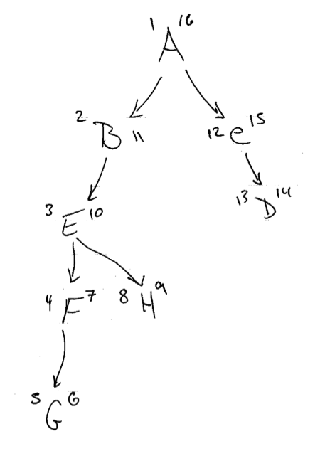
Pre-visit and Post-visit
Upon pre-visit and post-visit we can track how many visits we have done (u,v). These numbers are used to determine facts about the hierarchy of the graph. Given two nodes, if (u,v) of node 1 are between (u,v) of node 2, then node 1 is a child node (and vice versa).
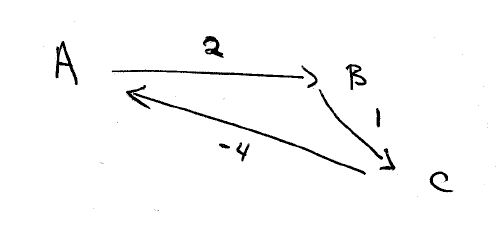
Types of Edges found by DFS
- forward edges: lead from a node to a non-child descendant
- back edges: lead to an ancestor in the DFS tree
- cross edges: lead to neither a descendant nor ancestor, but a node that has already been explored (?)
Sources & Sinks
A source is a node with no incoming edges. Conversely, a sink is a node with no outgoing edges. A directed acyclic graph must have these.
Directed Acyclic Graphs (DAGs)
- is a DAG if the DFS revealed there to be no back edges
- every edge leads to a vertex with a lower post number
- every DAG has at least one source and one sink
Strongly connected components
Two nodes, $u$ and $v$, of a directed graph are connected if there is a path from $u$ to $v$ and a path from $v$ to $u$.
Algorithm for finding Strongly Connected Components
- Find $G^R$ (by reversing the edges of $G$)
- the highest post number is a sink
- Run a DFS on $G^R$ to find node with highest post number.
- Start DFS on $G$ (not reversed!) starting at the sink node found in #2. Do not update pre- and post-numbers this time. We will use the numbers captured in step #1. When we run out of nodes to traverse to, we have covered everything in the strongly connected component, then delete this component from the graph (how?)
- Move on to the node with the next highest post number that remains in $G$. This one must belong to the next sink
Pre and Post Numbers in a DAG (example)
Paths in Graphs
How to find the shortest path in a graph.
Breadth-first Search
Finds the distance from a starting node to other nodes, assuming they are each 1 unit of distance apart
Pseudo-code
				# Input: G = (V, E)
				# Output: typically no direct output, but we will
				# know the distance from s to each reachable vertex

				# initially set	every vertex distance to infinity
				for each u in V
					u.dist = INF

				#set our starting vertext to distance 0,
				# put it in the queue
				s.dist = 0
				Q = [s]

				# main part of the alg (not recursive)
				while Q is not empty
					# grab the first thing on the queue...
					u = Q.getFirst
					Q.removeFirst
					# iterate through all of its edges...
					for each edge e in u.edges
						# if the distance hasn't been found yet...
						if e.vertex.dist == INFINITY
							# add the vertex to the Q for next
							# iteration and set the distance of
							# this found vertex
							inject(Q, e.vertex)
							e.vertex.dist = u.dist + 1
Dijkstra's Algorithm
Finds the shortest distance from a starting node to other nodes, for nodes that are any distance apart. Cannot handle graphs that have edges with negative weights.
					# Input: G = (V, E)
					# Output: we will know the shortest
					# distance from s to each reachable vertex

					# initial assumption values
					for each u in V
						u.dist = INFINITY
						u.prev = NIL

					# starting point distance is obviously 0
					s.dist = 0

					# using distance values as keys
					H = makequeue(V)
					while !H.isEmpty
						u = deletemin(H)
						for each edge e in u.edges
							if v.dist > u.dist + length(u,v)
								v.dist = u.dist + length(u,v)
								v.prev = u
								decreasekey(H,v)
Bellman Ford
Finds the shortest path in a graph. Can handle graphs with edges that have negative weights (whereas Dijkstra's cannot), and also detects negative cycles. O(|V| + |E|)
					# Input: G = (V, E), and no negative cycles
					# Output: we will know the shortest distance
					# from s to each reachable vertex

					# initial assumption values
					for each u in V
						u.dist = INFINITY
						u.prev = NIL

					s.dist = 0	# starting point distance is obviously 0

					# update distances and previous nodes
					for i = 1 to V.length -1
						for each edge e in G.edges
							update(e)

					# indicate if a negative cycle is found
					for each edge e in G.edges
							if e.endVertex.distance
								< e.startVertex.distance + e.weight
									return false

					def update(e)
						# here weight is same as length
						e.endVertex.distance = min(e.endVertex.distance,
						  e.startVertex.distance + e.weight)
						e.endVertex.prev = startVertex
					end

					return true
Dag shortest paths
Finds the shortest path in a Directed Acyclic Graph. O(|V| + |E|)
					# Input: G = (V, E),
					# Output: we will know the shortest distance
					# from s to each reachable vertex

					# initial assumption values
					for each u in V
						u.dist = INFINITY
						u.prev = NIL

					s.dist = 0  # starting point distance is obviously 0
					g.linearize
					for each vertex u in G.linearizedVerticies
						for each edge e in u.edges
							update(e)

					def update(e)
						# here weight is same as length
						e.endVertex.distance = min(e.endVertex.distance,
						  e.startVertex.distance + e.weight)
					end
Greedy Algorithms
Greedy algorithms build up a solution piece by piece, always choosing the next piece that offers the most obvious and immediate benefit. This can be an optimal approach, but not always.
Minimum Spanning Trees
Given an undirected graph, the minimum spanning tree is a tree representation of the graph which is fully connected and has the least weight possible
Kruskal's Algorithm for finding MST
Kruskal's algorithm for finding MST starts with an empty graph then repeatedly selects the next lightest edge that doesn't produce a cycle. This algorithm is greedy because it makes the most obvious decision at each step without looking ahead
				#input: a connected unirected graph with
				#weighted edges
				#output: a minimum spanning tree defined
				# by the edges X

				foreach u in V
					u.makeset
				X = []

				# sort increasing
				var sortedEdges = sortByWeight(self.edges)
				foreach edge {u,v} in sortedEdges
					if u.root != v.root
						X.add({u,v})
						union(u, v)
Prim's Algorithm for finding MST
Prim's algorithm also finds the minimum spanning tree, but the algorithm approach is similar to Dijkstra's algorithm. Here is a discussion of the differences.
				#input: a connected undirected graph with
				# weighted edges
				#output: a minimum spanning tree defined
				# by the edges X

				foreach u in V
					u.cost = INFINITY
					u.previous = nil
				#pick any initial node u0
				u0.cost = 0

				H = makequeue(V)
				while !H.isEmpty
					v = deletemin(H)
					for each edge {v,z} in E
						if (z.cost > G.weights(v,z))
							z.cost = G.weights(v,z)
							z.previous = v
Huffman Encoding
Compression encoding; replace byte values with the smallest possible bit-encoding from the most frequently used byte value to the least. See Standish Data Structures for a good example.
Proof Techniques
Invariants
Class Invariants: true after the object is created and after every method call
Loop Invariants: true before after and at the top of each iteration
Mathematical Induction
Weakest Precondition
Dynamic Programming
Doing things in a particular order so that you can make use of sub-problem solutions in subsequent steps.
Edit Distance
The cost or distance between two strings, in terms of inserts, substitutions, and deletes.
			From: S _ N O W Y
			To:   S U N N _ Y
The above "snowy" to "sunny" has an edit distance of 3 due to 1 insert (U), 1 replacement (O with N), and 1 delete (W). Solving more generally involves breaking each column examination into 3 sub-problems. Given the current subproblem matrix of E, the "best" choice is as follows:
E(i,j) = min{1 + E(i-1, j), 1 + E(i, j-1), diff(i,j) + E(i - 1, j - 1)}
Where diff is 0 if x[i] == y[j] else 1
Knapsack Problem
With Repetition
Without Repetition
Chain Matrix Multiplication
Find the optimal order of multiplication of matrices